GKD-BT Solo Confirmation Simple Backtest [Loxx]Giga Kaleidoscope GKD-BT Solo Confirmation Simple Backtest is a Backtesting module included in Loxx's "Giga Kaleidoscope Modularized Trading System".
█ GKD-BT Solo Confirmation Simple Backtest
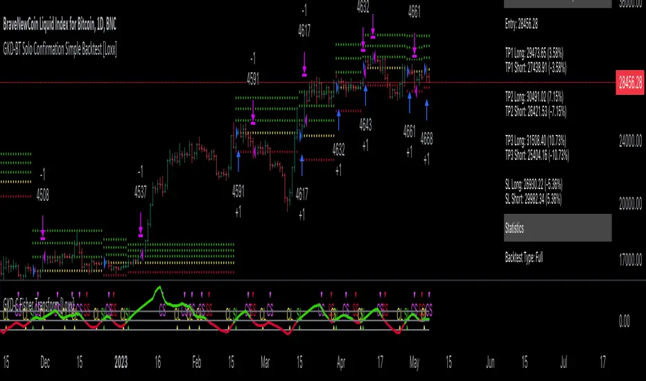
The Solo Confirmation Simple Backtest module enables users to perform Standard Long and Short signals on GKD-C confirmation indicators. This module represents the simplest form of Backtest in the GKD trading system. It includes two types of backtests: Trading and Full. The Trading backtest allows users to test individual trades, both long and short, one at a time. On the other hand, the Full backtest allows users to test either longs or shorts by toggling between them in the settings to view the results for each signal type. The Trading backtest simulates real trading, while the Full backtest tests all signals, whether long or short.
Additionally, this backtest module provides the option to test the GKD-C indicator with 1 to 3 take profits and 1 stop loss. The Trading backtest allows for the use of 1 to 3 take profits, while the Full backtest is limited to 1 take profit. The Trading backtest also offers the capability to apply a trailing take profit.
In terms of the percentage of trade removed at each take profit, this backtest module has the following hardcoded values:
Take profit 1: 50% of the trade is removed
Take profit 2: 25% of the trade is removed
Take profit 3: 25% of the trade is removed
Stop loss: 100% of the trade is removed
After each take profit is achieved, the stop loss level is adjusted. When take profit 1 is reached, the stop loss is moved to the entry point. Similarly, when take profit 2 is reached, the stop loss is shifted to take profit 1. The trailing take profit feature comes into play after take profit 2 or take profit 3, depending on the number of take profits selected in the settings. The trailing take profit is always activated on the final take profit when 2 or more take profits are chosen.
The backtest also offers the capability to restrict by a specific date range, allowing for simulated forward testing based on past data. Additionally, users have the option to display or hide a trading panel that provides relevant information about the backtest, statistics, and the current trade. It is also possible to activate alerts and toggle sections of the trading panel on or off. On the chart, historical take profit and stop loss levels are represented by horizontal lines overlaid for reference.
The GKD system utilizes volatility-based take profits and stop losses. Each take profit and stop loss is calculated as a multiple of volatility. You can change the values of the multipliers in the settings as well.
To utilize this strategy, follow these steps:
1. Adjust the "Confirmation Type" in the GKD-C Confirmation Indicator to "GKD New."
2. Import the value "Input into NEW GKD-BT Backtest" into the GKD-BT Solo Confirmation Simple Backtest module (this strategy backtest).
**The GKD-BT Solo Confirmation Simple Backtest module exclusively supports Standard Entries, both Long and Short. However, please note that this module uses a modified version of the standard entry, where long and short signals are directly imported from the Confirmation indicator without any baseline or volatility filtering applied.**
Volatility Types Included
17 types of volatility are included in this indicator
Close-to-Close
Parkinson
Garman-Klass
Rogers-Satchell
Yang-Zhang
Garman-Klass-Yang-Zhang
Exponential Weighted Moving Average
Standard Deviation of Log Returns
Pseudo GARCH(2,2)
Average True Range
True Range Double
Standard Deviation
Adaptive Deviation
Median Absolute Deviation
Efficiency-Ratio Adaptive ATR
Mean Absolute Deviation
Static Percent
Close-to-Close
Close-to-Close volatility is a classic and widely used volatility measure, sometimes referred to as historical volatility.
Volatility is an indicator of the speed of a stock price change. A stock with high volatility is one where the price changes rapidly and with a larger amplitude. The more volatile a stock is, the riskier it is.
Close-to-close historical volatility is calculated using only a stock's closing prices. It is the simplest volatility estimator. However, in many cases, it is not precise enough. Stock prices could jump significantly during a trading session and return to the opening value at the end. That means that a considerable amount of price information is not taken into account by close-to-close volatility.
Despite its drawbacks, Close-to-Close volatility is still useful in cases where the instrument doesn't have intraday prices. For example, mutual funds calculate their net asset values daily or weekly, and thus their prices are not suitable for more sophisticated volatility estimators.
Parkinson
Parkinson volatility is a volatility measure that uses the stock’s high and low price of the day.
The main difference between regular volatility and Parkinson volatility is that the latter uses high and low prices for a day, rather than only the closing price. This is useful as close-to-close prices could show little difference while large price movements could have occurred during the day. Thus, Parkinson's volatility is considered more precise and requires less data for calculation than close-to-close volatility.
One drawback of this estimator is that it doesn't take into account price movements after the market closes. Hence, it systematically undervalues volatility. This drawback is addressed in the Garman-Klass volatility estimator.
Garman-Klass
Garman-Klass is a volatility estimator that incorporates open, low, high, and close prices of a security.
Garman-Klass volatility extends Parkinson's volatility by taking into account the opening and closing prices. As markets are most active during the opening and closing of a trading session, it makes volatility estimation more accurate.
Garman and Klass also assumed that the process of price change follows a continuous diffusion process (Geometric Brownian motion). However, this assumption has several drawbacks. The method is not robust for opening jumps in price and trend movements.
Despite its drawbacks, the Garman-Klass estimator is still more effective than the basic formula since it takes into account not only the price at the beginning and end of the time interval but also intraday price extremes.
Researchers Rogers and Satchell have proposed a more efficient method for assessing historical volatility that takes into account price trends. See Rogers-Satchell Volatility for more detail.
Rogers-Satchell
Rogers-Satchell is an estimator for measuring the volatility of securities with an average return not equal to zero.
Unlike Parkinson and Garman-Klass estimators, Rogers-Satchell incorporates a drift term (mean return not equal to zero). As a result, it provides better volatility estimation when the underlying is trending.
The main disadvantage of this method is that it does not take into account price movements between trading sessions. This leads to an underestimation of volatility since price jumps periodically occur in the market precisely at the moments between sessions.
A more comprehensive estimator that also considers the gaps between sessions was developed based on the Rogers-Satchel formula in the 2000s by Yang-Zhang. See Yang Zhang Volatility for more detail.
Yang-Zhang
Yang Zhang is a historical volatility estimator that handles both opening jumps and the drift and has a minimum estimation error.
Yang-Zhang volatility can be thought of as a combination of the overnight (close-to-open volatility) and a weighted average of the Rogers-Satchell volatility and the day’s open-to-close volatility. It is considered to be 14 times more efficient than the close-to-close estimator.
Garman-Klass-Yang-Zhang
Garman-Klass-Yang-Zhang (GKYZ) volatility estimator incorporates the returns of open, high, low, and closing prices in its calculation.
GKYZ volatility estimator takes into account overnight jumps but not the trend, i.e., it assumes that the underlying asset follows a Geometric Brownian Motion (GBM) process with zero drift. Therefore, the GKYZ volatility estimator tends to overestimate the volatility when the drift is different from zero. However, for a GBM process, this estimator is eight times more efficient than the close-to-close volatility estimator.
Exponential Weighted Moving Average
The Exponentially Weighted Moving Average (EWMA) is a quantitative or statistical measure used to model or describe a time series. The EWMA is widely used in finance, with the main applications being technical analysis and volatility modeling.
The moving average is designed such that older observations are given lower weights. The weights decrease exponentially as the data point gets older – hence the name exponentially weighted.
The only decision a user of the EWMA must make is the parameter lambda. The parameter decides how important the current observation is in the calculation of the EWMA. The higher the value of lambda, the more closely the EWMA tracks the original time series.
Standard Deviation of Log Returns
This is the simplest calculation of volatility. It's the standard deviation of ln(close/close(1)).
Pseudo GARCH(2,2)
This is calculated using a short- and long-run mean of variance multiplied by ?.
?avg(var;M) + (1 ? ?) avg(var;N) = 2?var/(M+1-(M-1)L) + 2(1-?)var/(M+1-(M-1)L)
Solving for ? can be done by minimizing the mean squared error of estimation; that is, regressing L^-1var - avg(var; N) against avg(var; M) - avg(var; N) and using the resulting beta estimate as ?.
Average True Range
The average true range (ATR) is a technical analysis indicator, introduced by market technician J. Welles Wilder Jr. in his book New Concepts in Technical Trading Systems, that measures market volatility by decomposing the entire range of an asset price for that period.
The true range indicator is taken as the greatest of the following: current high less the current low; the absolute value of the current high less the previous close; and the absolute value of the current low less the previous close. The ATR is then a moving average, generally using 14 days, of the true ranges.
True Range Double
A special case of ATR that attempts to correct for volatility skew.
Standard Deviation
Standard deviation is a statistic that measures the dispersion of a dataset relative to its mean and is calculated as the square root of the variance. The standard deviation is calculated as the square root of variance by determining each data point's deviation relative to the mean. If the data points are further from the mean, there is a higher deviation within the data set; thus, the more spread out the data, the higher the standard deviation.
Adaptive Deviation
By definition, the Standard Deviation (STD, also represented by the Greek letter sigma ? or the Latin letter s) is a measure that is used to quantify the amount of variation or dispersion of a set of data values. In technical analysis, we usually use it to measure the level of current volatility.
Standard Deviation is based on Simple Moving Average calculation for mean value. This version of standard deviation uses the properties of EMA to calculate what can be called a new type of deviation, and since it is based on EMA, we can call it EMA deviation. Additionally, Perry Kaufman's efficiency ratio is used to make it adaptive (since all EMA type calculations are nearly perfect for adapting).
The difference when compared to the standard is significant--not just because of EMA usage, but the efficiency ratio makes it a "bit more logical" in very volatile market conditions.
Median Absolute Deviation
The median absolute deviation is a measure of statistical dispersion. Moreover, the MAD is a robust statistic, being more resilient to outliers in a data set than the standard deviation. In the standard deviation, the distances from the mean are squared, so large deviations are weighted more heavily, and thus outliers can heavily influence it. In the MAD, the deviations of a small number of outliers are irrelevant.
Because the MAD is a more robust estimator of scale than the sample variance or standard deviation, it works better with distributions without a mean or variance, such as the Cauchy distribution.
Efficiency-Ratio Adaptive ATR
Average True Range (ATR) is a widely used indicator for many occasions in technical analysis. It is calculated as the RMA of the true range. This version adds a "twist": it uses Perry Kaufman's Efficiency Ratio to calculate adaptive true range.
Mean Absolute Deviation
The mean absolute deviation (MAD) is a measure of variability that indicates the average distance between observations and their mean. MAD uses the original units of the data, which simplifies interpretation. Larger values signify that the data points spread out further from the average. Conversely, lower values correspond to data points bunching closer to it. The mean absolute deviation is also known as the mean deviation and average absolute deviation.
This definition of the mean absolute deviation sounds similar to the standard deviation (SD). While both measure variability, they have different calculations. In recent years, some proponents of MAD have suggested that it replace the SD as the primary measure because it is a simpler concept that better fits real life.
Static Percent
Static Percent allows the user to insert their own constant percent that will then be used to create take profits and stoploss
█ Giga Kaleidoscope Modularized Trading System
Core components of an NNFX algorithmic trading strategy
The NNFX algorithm is built on the principles of trend, momentum, and volatility. There are six core components in the NNFX trading algorithm:
1. Volatility - price volatility; e.g., Average True Range, True Range Double, Close-to-Close, etc.
2. Baseline - a moving average to identify price trend
3. Confirmation 1 - a technical indicator used to identify trends
4. Confirmation 2 - a technical indicator used to identify trends
5. Continuation - a technical indicator used to identify trends
6. Volatility/Volume - a technical indicator used to identify volatility/volume breakouts/breakdown
7. Exit - a technical indicator used to determine when a trend is exhausted
What is Volatility in the NNFX trading system?
In the NNFX (No Nonsense Forex) trading system, ATR (Average True Range) is typically used to measure the volatility of an asset. It is used as a part of the system to help determine the appropriate stop loss and take profit levels for a trade. ATR is calculated by taking the average of the true range values over a specified period.
True range is calculated as the maximum of the following values:
-Current high minus the current low
-Absolute value of the current high minus the previous close
-Absolute value of the current low minus the previous close
ATR is a dynamic indicator that changes with changes in volatility. As volatility increases, the value of ATR increases, and as volatility decreases, the value of ATR decreases. By using ATR in NNFX system, traders can adjust their stop loss and take profit levels according to the volatility of the asset being traded. This helps to ensure that the trade is given enough room to move, while also minimizing potential losses.
Other types of volatility include True Range Double (TRD), Close-to-Close, and Garman-Klass
What is a Baseline indicator?
The baseline is essentially a moving average, and is used to determine the overall direction of the market.
The baseline in the NNFX system is used to filter out trades that are not in line with the long-term trend of the market. The baseline is plotted on the chart along with other indicators, such as the Moving Average (MA), the Relative Strength Index (RSI), and the Average True Range (ATR).
Trades are only taken when the price is in the same direction as the baseline. For example, if the baseline is sloping upwards, only long trades are taken, and if the baseline is sloping downwards, only short trades are taken. This approach helps to ensure that trades are in line with the overall trend of the market, and reduces the risk of entering trades that are likely to fail.
By using a baseline in the NNFX system, traders can have a clear reference point for determining the overall trend of the market, and can make more informed trading decisions. The baseline helps to filter out noise and false signals, and ensures that trades are taken in the direction of the long-term trend.
What is a Confirmation indicator?
Confirmation indicators are technical indicators that are used to confirm the signals generated by primary indicators. Primary indicators are the core indicators used in the NNFX system, such as the Average True Range (ATR), the Moving Average (MA), and the Relative Strength Index (RSI).
The purpose of the confirmation indicators is to reduce false signals and improve the accuracy of the trading system. They are designed to confirm the signals generated by the primary indicators by providing additional information about the strength and direction of the trend.
Some examples of confirmation indicators that may be used in the NNFX system include the Bollinger Bands, the MACD (Moving Average Convergence Divergence), and the MACD Oscillator. These indicators can provide information about the volatility, momentum, and trend strength of the market, and can be used to confirm the signals generated by the primary indicators.
In the NNFX system, confirmation indicators are used in combination with primary indicators and other filters to create a trading system that is robust and reliable. By using multiple indicators to confirm trading signals, the system aims to reduce the risk of false signals and improve the overall profitability of the trades.
What is a Continuation indicator?
In the NNFX (No Nonsense Forex) trading system, a continuation indicator is a technical indicator that is used to confirm a current trend and predict that the trend is likely to continue in the same direction. A continuation indicator is typically used in conjunction with other indicators in the system, such as a baseline indicator, to provide a comprehensive trading strategy.
What is a Volatility/Volume indicator?
Volume indicators, such as the On Balance Volume (OBV), the Chaikin Money Flow (CMF), or the Volume Price Trend (VPT), are used to measure the amount of buying and selling activity in a market. They are based on the trading volume of the market, and can provide information about the strength of the trend. In the NNFX system, volume indicators are used to confirm trading signals generated by the Moving Average and the Relative Strength Index. Volatility indicators include Average Direction Index, Waddah Attar, and Volatility Ratio. In the NNFX trading system, volatility is a proxy for volume and vice versa.
By using volume indicators as confirmation tools, the NNFX trading system aims to reduce the risk of false signals and improve the overall profitability of trades. These indicators can provide additional information about the market that is not captured by the primary indicators, and can help traders to make more informed trading decisions. In addition, volume indicators can be used to identify potential changes in market trends and to confirm the strength of price movements.
What is an Exit indicator?
The exit indicator is used in conjunction with other indicators in the system, such as the Moving Average (MA), the Relative Strength Index (RSI), and the Average True Range (ATR), to provide a comprehensive trading strategy.
The exit indicator in the NNFX system can be any technical indicator that is deemed effective at identifying optimal exit points. Examples of exit indicators that are commonly used include the Parabolic SAR, the Average Directional Index (ADX), and the Chandelier Exit.
The purpose of the exit indicator is to identify when a trend is likely to reverse or when the market conditions have changed, signaling the need to exit a trade. By using an exit indicator, traders can manage their risk and prevent significant losses.
In the NNFX system, the exit indicator is used in conjunction with a stop loss and a take profit order to maximize profits and minimize losses. The stop loss order is used to limit the amount of loss that can be incurred if the trade goes against the trader, while the take profit order is used to lock in profits when the trade is moving in the trader's favor.
Overall, the use of an exit indicator in the NNFX trading system is an important component of a comprehensive trading strategy. It allows traders to manage their risk effectively and improve the profitability of their trades by exiting at the right time.
How does Loxx's GKD (Giga Kaleidoscope Modularized Trading System) implement the NNFX algorithm outlined above?
Loxx's GKD v2.0 system has five types of modules (indicators/strategies). These modules are:
1. GKD-BT - Backtesting module (Volatility, Number 1 in the NNFX algorithm)
2. GKD-B - Baseline module (Baseline and Volatility/Volume, Numbers 1 and 2 in the NNFX algorithm)
3. GKD-C - Confirmation 1/2 and Continuation module (Confirmation 1/2 and Continuation, Numbers 3, 4, and 5 in the NNFX algorithm)
4. GKD-V - Volatility/Volume module (Confirmation 1/2, Number 6 in the NNFX algorithm)
5. GKD-E - Exit module (Exit, Number 7 in the NNFX algorithm)
(additional module types will added in future releases)
Each module interacts with every module by passing data to A backtest module wherein the various components of the GKD system are combined to create a trading signal.
That is, the Baseline indicator passes its data to Volatility/Volume. The Volatility/Volume indicator passes its values to the Confirmation 1 indicator. The Confirmation 1 indicator passes its values to the Confirmation 2 indicator. The Confirmation 2 indicator passes its values to the Continuation indicator. The Continuation indicator passes its values to the Exit indicator, and finally, the Exit indicator passes its values to the Backtest strategy.
This chaining of indicators requires that each module conform to Loxx's GKD protocol, therefore allowing for the testing of every possible combination of technical indicators that make up the six components of the NNFX algorithm.
What does the application of the GKD trading system look like?
Example trading system:
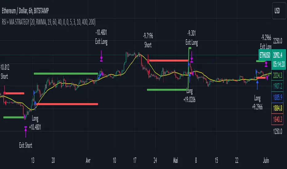
Backtest: Solo Confirmation Simple Backtest as shown on the chart above
Baseline: Hull Moving Average
Volatility/Volume: Hurst Exponent
Confirmation 1: Fisher Trasnform as shown on the chart above
Confirmation 2: Williams Percent Range
Continuation: Volatility-Adaptive Rapid RSI T3
Exit: Rex Oscillator
Each GKD indicator is denoted with a module identifier of either: GKD-BT, GKD-B, GKD-C, GKD-V, or GKD-E. This allows traders to understand to which module each indicator belongs and where each indicator fits into the GKD system.
Giga Kaleidoscope Modularized Trading System Signals (based on the NNFX algorithm)
Standard Entry
1. GKD-C Confirmation 1 Signal
2. GKD-B Baseline agrees
3. Price is within a range of 0.2x Volatility and 1.0x Volatility of the Goldie Locks Mean
4. GKD-C Confirmation 2 agrees
5. GKD-V Volatility/Volume agrees
Baseline Entry
1. GKD-B Baseline signal
2. GKD-C Confirmation 1 agrees
3. Price is within a range of 0.2x Volatility and 1.0x Volatility of the Goldie Locks Mean
4. GKD-C Confirmation 2 agrees
5. GKD-V Volatility/Volume agrees
6. GKD-C Confirmation 1 signal was less than 7 candles prior
Volatility/Volume Entry
1. GKD-V Volatility/Volume signal
2. GKD-C Confirmation 1 agrees
3. Price is within a range of 0.2x Volatility and 1.0x Volatility of the Goldie Locks Mean
4. GKD-C Confirmation 2 agrees
5. GKD-B Baseline agrees
6. GKD-C Confirmation 1 signal was less than 7 candles prior
Continuation Entry
1. Standard Entry, Baseline Entry, or Pullback; entry triggered previously
2. GKD-B Baseline hasn't crossed since entry signal trigger
3. GKD-C Confirmation Continuation Indicator signals
4. GKD-C Confirmation 1 agrees
5. GKD-B Baseline agrees
6. GKD-C Confirmation 2 agrees
1-Candle Rule Standard Entry
1. GKD-C Confirmation 1 signal
2. GKD-B Baseline agrees
3. Price is within a range of 0.2x Volatility and 1.0x Volatility of the Goldie Locks Mean
Next Candle:
1. Price retraced (Long: close < close or Short: close > close )
2. GKD-B Baseline agrees
3. GKD-C Confirmation 1 agrees
4. GKD-C Confirmation 2 agrees
5. GKD-V Volatility/Volume agrees
1-Candle Rule Baseline Entry
1. GKD-B Baseline signal
2. GKD-C Confirmation 1 agrees
3. Price is within a range of 0.2x Volatility and 1.0x Volatility of the Goldie Locks Mean
4. GKD-C Confirmation 1 signal was less than 7 candles prior
Next Candle:
1. Price retraced (Long: close < close or Short: close > close )
2. GKD-B Baseline agrees
3. GKD-C Confirmation 1 agrees
4. GKD-C Confirmation 2 agrees
5. GKD-V Volatility/Volume Agrees
1-Candle Rule Volatility/Volume Entry
1. GKD-V Volatility/Volume signal
2. GKD-C Confirmation 1 agrees
3. Price is within a range of 0.2x Volatility and 1.0x Volatility of the Goldie Locks Mean
4. GKD-C Confirmation 1 signal was less than 7 candles prior
Next Candle:
1. Price retraced (Long: close < close or Short: close > close)
2. GKD-B Volatility/Volume agrees
3. GKD-C Confirmation 1 agrees
4. GKD-C Confirmation 2 agrees
5. GKD-B Baseline agrees
PullBack Entry
1. GKD-B Baseline signal
2. GKD-C Confirmation 1 agrees
3. Price is beyond 1.0x Volatility of Baseline
Next Candle:
1. Price is within a range of 0.2x Volatility and 1.0x Volatility of the Goldie Locks Mean
2. GKD-C Confirmation 1 agrees
3. GKD-C Confirmation 2 agrees
4. GKD-V Volatility/Volume Agrees
Strategia Pine Script®